Understanding DEMs, DSMs, and DTMs: A Complete Guide to Digital Elevation Data
Learn the key differences between DEMs, DSMs, and DTMs, how they're created, their applications, and how to choose the right elevation data for your project.
Summary
- What DEMs are: Raster grids representing Earth’s surface elevation, where each pixel contains an elevation value normalized to a datum (typically mean sea level)
- Three types: DEM is an umbrella term encompassing Digital Surface Models (DSMs) that include all objects, and Digital Terrain Models (DTMs) that show only bare-earth
- Creation methods: InSAR (radar interferometry), stereo photogrammetry (multiple optical angles), LiDAR (laser scanning), contour digitization, and ground surveys
- Key applications: Flood modeling, urban planning, infrastructure design, mining volumetrics, hydrology analysis, environmental monitoring, and disaster response
- Accuracy factors: Spatial resolution, vertical resolution, acquisition method, temporal currency, and processing algorithms all affect DEM quality
- Data sources: Free global datasets (SRTM, ASTER, ALOS) serve many applications, while commercial high-resolution options deliver sub-meter accuracy for critical projects
- Need high-quality DEMs? Contact Geopera to access stereoscopic satellite imagery for custom DEM generation or discuss which elevation data source best fits your project requirements
Our planet is full of peaks, valleys, natural habitats, and human-made structures. Digital elevation data brings these highs, lows, and features into sharp focus.
By visualizing landscapes as elevation data, you can estimate areas vulnerable to sea-level rise, detect vegetation encroachment, identify optimal infrastructure routes, and solve problems ranging from flood risk assessment to mine planning.
There are multiple ways to model elevation, and the terminology can be confusing. The term Digital Elevation Model (DEM) is often used as a blanket term, but it encompasses distinct product types—Digital Surface Models (DSMs) and Digital Terrain Models (DTMs)—each serving different purposes.
Understanding these differences is crucial for selecting the right elevation data for your application.
What Are Digital Elevation Models?
A Digital Elevation Model, also known as a DEM, is a raster GIS layer representing the Earth’s surface as a pixel grid. Each pixel in this grid contains an elevation value that indicates the height of that location above a reference point.
These elevation values are normalized to a vertical datum—a standardized reference for zero elevation, typically based on mean sea level. This consistent reference point allows elevation data from different sources and times to be compared and analyzed together.
The term DEM is commonly used as an umbrella term encompassing both Digital Surface Models and Digital Terrain Models, which we’ll explore in detail below. In practice, when working with coarser-resolution global datasets that can’t distinguish individual buildings or trees, the generic term DEM is most appropriate.
DEMs are stored in various file formats including GeoTIFF (.tif), the USGS DEM format (.dem), binary float files (.flt), and text-based ASCII grids (.asc). The GeoTIFF format has become the de facto standard due to its wide software support and ability to embed georeferencing information directly in the file.
How Are DEMs Created?
To capture elevation data, a single standard optical image isn’t sufficient. You need a way to capture depth. Here are the primary methods used to create digital elevation models:
SAR Interferometry (InSAR)
This method uses synthetic aperture radar (SAR) to collect multiple radar images of the same area from different angles, building a 3D representation through phase difference analysis.
SAR sensors emit microwave pulses and measure the reflected signal. By comparing the phase differences between two radar images captured from slightly different positions, interferometric algorithms can calculate the distance from the sensor to each point on the ground—revealing elevation.
The key advantage of InSAR is its ability to work in all weather conditions, day or night, since radar penetrates clouds. The Shuttle Radar Topography Mission (SRTM) used this technique during its 11-day mission in 2000 to map most of Earth’s landmass.
Stereo Photogrammetry
Similar to InSAR but using optical sensors, stereo photogrammetry captures multiple images of the same area from different angles to extract 3D information. This can be accomplished using satellite, aerial, or drone-based platforms.
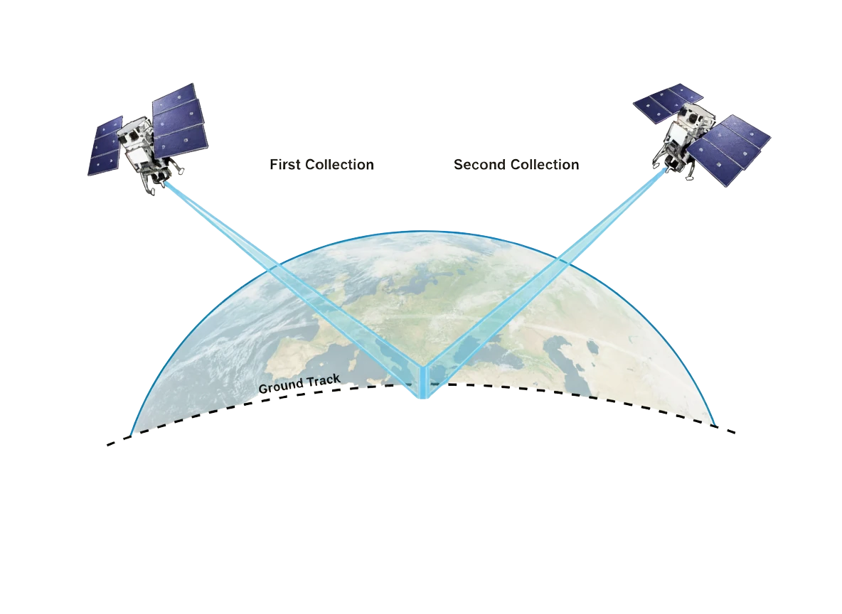 Stereoscopic collection captures the same location from two different viewing angles, creating the geometric conditions necessary to extract precise elevation data.
Modern high-resolution satellites like WorldView-2 and WorldView-3 excel at stereo DEM generation through in-track stereo collection, where both images are captured during a single orbital pass within 45-90 seconds of each other. This temporal consistency—where ground conditions remain nearly identical between captures—improves the reliability of photogrammetric matching and the resulting elevation accuracy.
Learn more about how stereoscopic satellite imagery creates accurate 3D elevation models from paired 2D images.
LiDAR (Light Detection and Ranging)
LiDAR sensors actively fire laser pulses and measure the reflected light to determine the elevation of Earth’s surface. Instead of producing a raster grid directly, LiDAR typically creates a dense point cloud—millions of precisely positioned elevation measurements.
These point clouds can be converted into raster grids for easier processing and integration with other GIS data. LiDAR offers the highest spatial and vertical accuracy of any elevation capture method, with centimeter-level precision achievable under ideal conditions.
The trade-off is cost. While LiDAR is cost-effective for small critical areas, it becomes prohibitively expensive for large-scale regional mapping compared to satellite-based methods.
Digitizing Contour Lines
By using an existing topographic map with contour lines, you can extract elevation data using GIS software. This legacy method interpolates a continuous surface from the discrete contour elevations shown on the map.
While less accurate than modern sensing techniques, contour digitization remains useful for historical analysis and areas where no other elevation data exists.
Ground Surveying
Traditional surveying with theodolites and differential GPS involves assessing known XYZ positions and systematically measuring neighboring areas. This method requires skilled labor, substantial time investment, and very careful inputs to maintain accuracy.
Ground surveying delivers excellent accuracy but is only practical for small, critical areas where the investment is justified—such as engineering-grade surveys for major infrastructure projects.
What Are Digital Surface Models (DSMs)?
A Digital Surface Model captures the surface along with all natural and human-made structures—vegetation, buildings, power lines, and any other objects elevated above the ground.
In short: DSMs represent the ground AND everything on it.
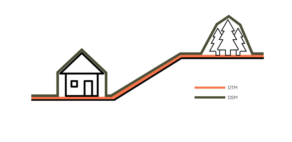 Figure: Comparison between DTM and DSM. DTMs represent the bare earth surface without buildings and vegetation, while DSMs include all objects on the terrain. Source: heliguy.com
DSMs capture the “first return” surface—the top of whatever is present when looking straight down from above. In a forest, this would be the tree canopy. In a city, this would be building rooftops. Only in open areas does the DSM show the actual ground surface.
Common Applications of DSMs
Because DSMs represent the surface and all of its above-ground features, they’re particularly valuable for:
Urban planning and 3D city modeling: DSMs provide the foundation for creating accurate 3D representations of cities, essential for visualization, planning, and analysis of urban development.
Runway approach zone analysis in aviation: Detecting the safest landing routes for aircraft requires knowing the height of all obstacles—buildings, trees, towers—in the approach corridor. DSMs excel at this application.
Building height extraction: By comparing a DSM with a bare-earth DTM of the same area, you can calculate precise building heights across entire urban areas.
Vegetation canopy height mapping: The difference between DSM and DTM reveals canopy height, critical for forestry management and biomass estimation.
Disaster management and damage assessment: Post-disaster DSMs can be compared with pre-event data to identify collapsed buildings, vegetation loss, and infrastructure damage.
Telecommunications line-of-sight planning: Planning microwave links and radio networks requires knowing exactly what obstacles exist between transmission points—a job perfectly suited to DSMs.
Solar panel placement optimization: DSMs combined with sun angle calculations identify roof areas with optimal solar exposure while accounting for shadowing from nearby buildings and trees.
What Are Digital Terrain Models (DTMs)?
Digital Terrain Models represent the bare-earth surface without natural or man-made features. All above-ground objects—trees, buildings, vehicles, power lines—are removed through processing, revealing only the underlying terrain.
The distinction between DTMs and DSMs becomes most evident in heavily developed urban areas with high-rise buildings. Places like Manhattan or Hong Kong Island have dramatically different surface and terrain elevations—the DSM captures skyscraper tops hundreds of meters above the DTM’s ground surface.
How DTMs Differ from DSMs
A critical point: DTMs can be derived from DSMs, but not the other way around.
Creating a DTM from a DSM requires sophisticated classification algorithms that identify and remove above-ground features while preserving the ground surface. This is considerably more complex than simply capturing the surface, which is why DTM production is more computationally intensive and often more expensive than DSM generation.
The nDSM Concept
The combination of DSM and DTM creates height information for above-ground features, known as a normalized Digital Surface Model (nDSM). The math is simple and intuitive:
DSM - DTM = nDSM
This normalized model shows the height of objects above the ground. A tree might appear as 15 meters in the nDSM, while a building shows its actual structural height rather than its absolute elevation.
nDSMs are particularly useful for:
- Forestry applications: Calculating tree heights across large forest areas
- Urban planning: Extracting building heights for zoning compliance and 3D modeling
- Vegetation management: Identifying power line encroachment risks
- Change detection: Tracking growth of vegetation or construction of new structures
Common Applications of DTMs
DTMs shine in applications where bare-earth elevation is essential:
Hydrology and watershed analysis: Water flows across the ground surface, not over tree canopies or building roofs. Accurate flow direction and accumulation modeling requires bare-earth DTMs.
Infrastructure routing: Planning roads, railways, pipelines, and power transmission lines requires knowing the actual ground elevation to calculate cut-and-fill volumes, assess slope stability, and optimize routes.
Flood modeling: Predicting flood inundation extents demands bare-earth elevation data. A DSM would incorrectly suggest that buildings block water flow, when in reality water flows around and through urban areas at ground level.
Geomorphology studies: Understanding landforms, erosion patterns, and geological processes requires seeing the actual terrain without the visual clutter of surface features.
Archaeological feature detection: Subtle terrain variations that indicate buried structures or historical earthworks are only visible in bare-earth DTMs, particularly those derived from LiDAR that penetrates vegetation.
Terrain-based military planning: Ground movement analysis, line-of-sight calculations for ground observers, and trafficability assessment all require accurate bare-earth terrain models.
DEM vs DSM vs DTM: Key Differences
Understanding the distinctions between these elevation model types is essential for selecting the right product for your application:
| Feature | DEM | DSM | DTM |
|---|---|---|---|
| Definition | Umbrella term for elevation data | Surface + all objects | Bare-earth only |
| Includes vegetation | Depends on product type | Yes | No |
| Includes buildings | Depends on product type | Yes | No |
| Best for hydrology | Only if it’s a DTM | No | Yes |
| Best for urban 3D | Only if it’s a DSM | Yes | No |
| Derivation | - | Direct from sensors | Requires classification |
| Processing complexity | - | Lower | Higher |
Quick Recap
- DEM: Generic term that could refer to either a DSM or DTM. Often used for coarse-resolution data where the distinction doesn’t matter.
- DSM: Everything visible from above—the canopy model showing tree tops, building roofs, and any other elevated features.
- DTM: Ground surface only, with all features removed through classification processing.
In practice, low-resolution global datasets (30m pixel size) don’t meaningfully distinguish between DSM and DTM because they can’t resolve individual trees and buildings anyway. The distinction becomes critical when working with high-resolution data where above-ground features are clearly visible.
DEM Quality and Accuracy
DEM accuracy is most commonly estimated by calculating the Root Mean Square Error (RMSE) of elevation—comparing DEM-derived heights against reference points with known elevations measured through precise ground surveys.
However, there’s much more to DEM quality than just vertical accuracy. Horizontal positional accuracy matters too, particularly when overlaying DEMs with other spatial data like imagery or vector features.
Factors Affecting DEM Quality
The quality of any digital elevation model depends on multiple interrelated factors:
1. Acquisition Method
Different elevation capture methods produce vastly different accuracy levels:
LiDAR: Best vertical accuracy, with 5-15cm precision achievable under ideal conditions. The active laser approach and dense point cloud output make this the gold standard for high-accuracy applications.
Stereo photogrammetry: Good accuracy, typically 30cm to 1m vertical precision with high-resolution satellites like WorldView-3. Accuracy depends heavily on image resolution, convergence angle between stereo pairs, and ground control points.
InSAR: Moderate accuracy, ranging from several meters to tens of meters depending on radar wavelength, baseline distance, and processing techniques. Excellent for large-area mapping where meter-level accuracy is sufficient.
Ground survey: Excellent accuracy but spatially limited. Practical only for small critical areas requiring engineering-grade precision.
2. Spatial Resolution
Spatial resolution is determined by the distance between sample points. This can be relatively uniform in stereo imagery, somewhat uniform in radar and LiDAR datasets, or highly variable in DEMs created from manual surveying methods.
Coarser resolution means small terrain features can’t be captured. A 30m resolution DEM will completely miss a 5m wide gully, while a 1m resolution model will capture it clearly.
3. Vertical Resolution
The vertical resolution of elevation data defines the possible height difference between the modeled elevation and the actual ground-truthed elevation of the surface.
This is often the most critical specification for applications like infrastructure design, where even small elevation errors can affect drainage patterns, cut-and-fill calculations, and slope stability assessments.
As a general hierarchy: LiDAR produces the best vertical resolution, followed by high-resolution stereo photogrammetry, then InSAR and lower-resolution optical stereo methods.
4. Temporal Resolution
One consideration often overlooked: How recently was the elevation data acquired?
This temporal resolution becomes particularly relevant for change detection applications or when using DSMs to study temporally variable features like vegetation growth or new construction. A 2000-vintage SRTM DEM won’t reflect the massive urban development that’s occurred in many cities over the past 25 years.
5. Error Sources
Multiple factors introduce errors during DEM acquisition and processing:
- Atmospheric and ionospheric interference: Affects radar and optical satellite observations, introducing phase delays (SAR) or image distortions (optical)
- Cloud cover: Completely blocks optical methods, creating data voids in stereo-derived DEMs
- Vegetation penetration: LiDAR often penetrates vegetation to reach the ground, while photogrammetry sees only the canopy top
- Co-registration errors: Misalignment between stereo image pairs degrades elevation extraction accuracy
- Processing artifacts: Interpolation errors, edge effects, and algorithm limitations introduce systematic biases
Vertical Errors in DEMs
Vertical errors typically manifest as two distinct feature types:
Sinks (also called depressions or pits): Areas surrounded by higher elevation values, representing internal drainage that may or may not be real. Some sinks are natural features, particularly in glacial or karst landscapes, but many result from DEM imperfections.
Peaks (also called spikes): Areas surrounded by cells of lower elevation. These are usually natural features and are less problematic for analysis than sinks.
The prevalence of sinks increases with coarser resolution. Often 1% of cells in a 30-meter resolution DEM consist of artificial sinks, increasing to 5% or more in three arc-second (approximately 90m) datasets.
Another common error type is striping artifacts—systematic patterns resulting from sampling errors during DEM creation. These are most noticeable in flat areas when elevation is stored as integer values rather than floating-point numbers.
Creating Depressionless DEMs
When faced with sinks in DEMs, it’s often necessary to remove or fill them to create a depressionless DEM. This is particularly critical for hydrological applications.
A DEM free of artificial sinks serves as the proper input for flow direction processing. Artificial sinks trap simulated water flow, leading to erroneous flow-direction rasters and incorrect watershed delineation.
Most GIS applications include tools to:
- Identify sinks and their spatial distribution
- Fill sinks to create continuous flow surfaces
- Calculate sink depth to distinguish real depressions from artifacts
This pre-processing step is essential before conducting any hydrological analysis with elevation data.
Common DEM Applications
DEMs serve critical functions across nearly every industry that works with spatial data. The vertical dimension unlocks analyses impossible with 2D imagery alone.
1. Hydrology and Flood Modeling
Water flows downhill—a simple fact that makes elevation data fundamental to all hydrological analysis.
DEMs enable:
- Flow direction and accumulation analysis: Determining the path water takes across a landscape and which areas contribute flow to specific points
- Watershed delineation: Automatically extracting drainage basin boundaries based on terrain
- Flood inundation mapping: Modeling which areas would flood under various water level scenarios, critical for sea-level rise planning and storm surge prediction
- Stream network extraction: Deriving channel networks from flow accumulation patterns
Accurate flood models require high-resolution, bare-earth DTMs. Research has shown that current global DEMs often fail to capture topographic details in floodplains, leading to significant errors in flood extent predictions. For critical flood risk assessment, commercial high-resolution DEMs or LiDAR-derived DTMs deliver the accuracy needed.
As our climate changes and sea levels rise, elevation-based coastal vulnerability assessment has become increasingly important for planning adaptation strategies.
2. Infrastructure Planning
Elevation data is fundamental to infrastructure route optimization and design.
DEMs support:
- Road, rail, and pipeline route optimization: Finding paths that minimize cut-and-fill requirements while avoiding excessive slopes
- Cut-and-fill volume calculations: Precisely quantifying earthwork requirements for construction planning and cost estimation
- Line-of-sight analysis: Determining visibility for telecommunications towers, ensuring clear signal paths
- Slope stability assessment: Identifying high-risk terrain where landslides or erosion could threaten infrastructure
Avoiding high-slope areas reduces both construction costs and environmental impacts. The ability to analyze thousands of potential route alternatives using elevation data leads to more efficient, sustainable infrastructure.
Explore how Geopera supports infrastructure applications with high-resolution satellite imagery and elevation data.
3. Mining Operations
The mining industry relies heavily on accurate, current elevation data for operational planning and regulatory compliance.
DEMs enable:
- Volumetric calculations for stockpiles and excavations: Accurately measuring ore, waste rock, and product volumes for inventory management and revenue calculation
- Pit progression monitoring: Tracking how excavations evolve over time, comparing planned vs. actual mining progress
- Haul road design: Optimizing road grades and routes to minimize fuel consumption and equipment wear
- Rehabilitation monitoring: Demonstrating compliance with environmental obligations by tracking restoration of disturbed areas
The temporal component is critical in mining. Time-series DEMs created from regular stereo satellite collections track volume changes with precision, providing the data needed for operational decisions and regulatory reporting.
Learn more about satellite imagery applications for mining operations.
4. Agriculture
Topography influences soil properties, water movement, and microclimate—making elevation data valuable for precision agriculture.
DEMs support:
- Topography-informed management zones: Dividing fields based on slope, aspect, and elevation to apply variable-rate inputs
- Drainage planning: Identifying low spots where water accumulates, informing tile drainage system design
- Erosion risk assessment: Calculating slope length and steepness factors for erosion prediction models
- Precision irrigation design: Optimizing sprinkler placement and flow rates based on topography
- Field-scale elevation mapping: Informing precision planting decisions, particularly for crops sensitive to waterlogging
Understanding field-scale topographic variation helps farmers optimize inputs, reduce costs, and minimize environmental impacts.
Discover how Geopera supports agriculture with satellite-derived insights.
5. Urban Planning
Cities exist in three dimensions, and elevation data brings that third dimension into planning workflows.
DEMs enable:
- 3D city modeling: Creating realistic urban visualizations for planning, public consultation, and design review
- Building height extraction: Deriving building heights by subtracting DTM from DSM
- Viewshed analysis: Determining what’s visible from specific locations, critical for visual impact studies of new developments
- Solar potential mapping: Identifying roof areas with optimal sun exposure while accounting for shadowing
- Green infrastructure design: Planning drainage solutions, green roofs, and urban forests with proper understanding of topography
6. Environmental Monitoring
Environmental applications span from disaster assessment to ecosystem management.
DEMs support:
- Landslide risk assessment and detection: Identifying unstable slopes and measuring terrain deformation after mass movement events
- Coastal erosion measurement: Quantifying beach and cliff elevation changes over time
- Forest canopy height modeling: Estimating biomass by calculating tree heights from DSM minus DTM
- Habitat mapping: Many species distributions correlate with topographic features like slope, aspect, and elevation
Explore Geopera’s capabilities for environmental monitoring applications.
7. Disaster Response
After earthquakes, landslides, volcanic eruptions, or major storms, elevation change detection reveals the extent and severity of impacts.
DEMs enable:
- Earthquake deformation mapping: Measuring ground surface changes caused by tectonic movement
- Landslide extent and volume calculation: Quantifying material movement for response planning
- Volcanic topographic change tracking: Monitoring lava dome growth or crater formation
- Infrastructure damage assessment: Identifying collapsed buildings, damaged roads, and altered drainage patterns
Rapid DEM generation from satellite stereo imagery collected immediately after disasters provides critical information for response efforts.
8. Archaeology
Bare-earth LiDAR DEMs have revolutionized archaeology by revealing subtle terrain features invisible under vegetation.
Applications include:
- Buried structure detection: Ancient building foundations, defensive earthworks, and agricultural terraces create subtle elevation variations visible in high-resolution DTMs
- Landscape reconstruction: Understanding historical environments and settlement patterns
- Site prospection: Identifying promising areas for investigation before expensive excavation
Famous examples include LiDAR revealing extensive Mayan cities beneath Central American jungle canopy—settlements that were completely invisible in conventional imagery.
9. Geologic Studies
Elevation patterns reveal Earth’s geological structure and active processes.
DEMs support:
- Tectonic feature identification: Fault scarps, rift valleys, and volcanic features are clearly visible in elevation data
- Fault mapping: Identifying and characterizing active faults for seismic hazard assessment
- Geomorphology analysis: Understanding how landscapes evolve through erosion, deposition, and tectonic processes
A compelling example: Digital elevation models of the East African Rift System clearly show the thermal bulges and grabens where the African continent is slowly splitting apart, eventually forming a new ocean.
10. Orthorectification
DEMs are required to remove terrain-induced distortions from satellite and aerial imagery, converting raw imagery into map-accurate products.
Without elevation data to account for terrain relief, imagery of mountainous areas shows geometric distortions where ridges appear to lean and valleys appear compressed. Orthorectification uses DEMs to model these distortions and remove them, producing imagery where every pixel is in its correct geographic position.
This is critical for:
- Creating seamless image mosaics
- Accurate distance and area measurements
- Change detection between images from different dates
- Overlaying imagery with other GIS data layers
Where to Find Elevation Data
There are plenty of places to find digital elevation models. From free satellite data to LiDAR sources, here’s how to find the elevation data you need.
Free Global Datasets
1. SRTM (Shuttle Radar Topography Mission)
During its 11-day mission in February 2000, the Space Shuttle Endeavour orbited Earth 16 times per day, systematically mapping the planet’s topography using interferometric synthetic aperture radar.
Coverage: Approximately 80% of Earth’s landmass (between 60°N and 56°S latitude)
Resolution: 1 arc-second (approximately 30 meters) globally; originally 90m outside the United States but 30m data now released worldwide
Method: InSAR with two radar antennas separated by a 60-meter mast
Vertical accuracy: Less than 16m absolute vertical error for most areas
Access: Free download from USGS Earth Explorer
Pros: Free, global, consistent methodology, well-documented accuracy, widely used as a baseline
Cons: Data from 2000 (now 25 years old), moderate resolution, data voids in challenging terrain like steep mountains, doesn’t reflect recent landscape changes
SRTM remains one of the most widely used global elevation datasets due to its consistent quality and complete documentation, despite its age.
2. ASTER GDEM (Global Digital Elevation Model)
The Advanced Spaceborne Thermal Emission and Reflection Radiometer (ASTER) is a joint operation by NASA and Japan’s Ministry of Economy, Trade, and Industry (METI). The ASTER Global Digital Elevation Model was generated from stereo pair images collected by the ASTER instrument aboard the Terra satellite.
Coverage: Approximately 80% of Earth (83°N to 83°S)
Resolution: 1 arc-second (approximately 30 meters)
Method: Stereo optical imagery from nadir and backward-looking telescopes
Versions: GDEM Version 2 (2011) and Version 3 (2019) with improved artifact correction and void filling
Access: Free download from NASA Earthdata and USGS Earth Explorer
Pros: Free, newer than SRTM in some areas, performs well in rugged mountainous terrain
Cons: Artifacts in persistently cloudy regions, variable accuracy due to cloud contamination during source image collection, can be less accurate than SRTM in flat areas
ASTER GDEM Version 3 represents significant improvements over earlier versions, with better handling of water bodies and reduced artifacts.
3. JAXA ALOS World 3D
ALOS World 3D is a global DSM dataset generated by the Japan Aerospace Exploration Agency (JAXA) from images collected by the Panchromatic Remote-sensing Instrument for Stereo Mapping (PRISM) aboard the Advanced Land Observing Satellite (ALOS).
Coverage: Global land area
Resolution: 30 meters (1 arc-second) freely available; 5-meter version available for some areas through commercial licensing
Method: PRISM stereo optical imagery
Acquisition period: 2006-2011
Access: Free registration required through JAXA’s Earth Observation Research Center portal
Pros: Good accuracy, more recent than SRTM, excellent void filling, better handling of steep terrain than ASTER
Cons: Requires registration, still approximately 15 years old, doesn’t reflect very recent landscape changes
The ALOS World 3D dataset has become increasingly popular as an alternative to SRTM and ASTER for applications requiring global coverage.
4. Regional LiDAR Sources
Many national, state, and local governments have invested in LiDAR collection and make the resulting elevation data freely available.
Examples include:
- USGS 3D Elevation Program (3DEP) covering the United States
- Environment Agency LiDAR data for England
- Australian state government programs (ELVIS portal provides unified access)
- Various European national mapping agencies
Characteristics: Highest accuracy of freely available options (often sub-meter vertical accuracy), typically bare-earth DTMs and surface DSMs both available, limited to specific geographic areas with government-funded collection
Access: Usually through government geospatial data portals
If you’re working in a developed country, it’s worth checking whether your local or regional government provides free LiDAR-derived DEMs. The accuracy is typically far superior to global satellite datasets.
Commercial High-Resolution Options
Free global datasets serve many applications well, but some projects require higher accuracy, more recent data, or specific product characteristics.
When Free Data Isn’t Enough
Consider commercial elevation data when you need:
- Current data for change detection: Comparing recent elevations against historical baselines to measure terrain changes
- Sub-meter vertical accuracy: Engineering-grade precision for critical infrastructure or regulatory compliance
- Specific coverage without data voids: Ensuring complete coverage of your area of interest
- Defined product type (DSM vs DTM): Many free datasets don’t clearly distinguish between surface and terrain models
Satellite-Derived DEMs
High-resolution satellites like WorldView-2 and WorldView-3 can collect stereoscopic imagery that, when processed photogrammetrically, produces DEMs with sub-meter vertical accuracy.
Characteristics:
- 50cm to 1m vertical accuracy achievable with proper ground control
- Custom tasking enables collection of current stereo pairs
- Large-area coverage possible (thousands of square kilometers)
- Both DSM and DTM products can be generated with appropriate processing
Geopera provides access to stereoscopic satellite imagery from the WorldView constellation, including existing archive data and custom tasking for new collections. Stereo pairs can be delivered for in-house DEM extraction or processed into elevation products by our partners.
Aerial LiDAR
For the highest accuracy requirements, aerial LiDAR collection remains the gold standard.
Characteristics:
- Centimeter-level vertical accuracy (5-15cm typical)
- Ultra-dense point clouds (10+ points per square meter)
- Simultaneous DTM and DSM generation
- Excellent vegetation penetration for ground extraction
Trade-offs:
- Expensive for large areas (costs scale with area)
- Requires specialized aircraft and equipment
- Weather-dependent collection
- Longer lead times for mobilization
Aerial LiDAR makes economic sense for critical infrastructure projects, detailed urban mapping, or smaller areas requiring engineering-grade accuracy.
Getting Help Choosing the Right Data
Not sure which elevation data source fits your project requirements?
Contact Geopera to discuss your specific needs. Our team can help you determine whether free global datasets, commercial satellite-derived DEMs, or custom stereo tasking best meets your accuracy, spatial coverage, temporal requirements, and budget constraints.
We can provide:
- Assessment of existing elevation data coverage and quality for your area of interest
- Access to archive stereoscopic satellite imagery for photogrammetric DEM extraction
- Coordination of custom stereo collection missions
- Connections to processing partners for DEM generation services
Working with DEM Data
Once you’ve acquired elevation data, you’ll need appropriate tools to open, visualize, analyze, and extract insights from it.
File Formats
DEMs are distributed in various file formats, each with different characteristics:
GeoTIFF (.tif): The most common format, widely supported across GIS platforms. Embeds georeferencing information within the file, simplifying data management. Can store elevation as integer or floating-point values.
USGS DEM (.dem): Legacy format from the U.S. Geological Survey. Less common now but still encountered in older datasets.
Float (.flt): Binary raster format storing elevation as floating-point values, often paired with a header file (.hdr) containing georeferencing information.
ASCII Grid (.asc): Text-based format where elevation values are stored as readable numbers in a grid structure. Human-readable but inefficient for large datasets.
Point Clouds (.las, .laz): LiDAR’s native format stores irregular point measurements rather than regular grids. LAZ is a compressed version of LAS. These require conversion to raster DEMs for most GIS analysis workflows.
Software Tools
You’ll need Geographic Information System (GIS) software or specialized applications to work with elevation data, as DEMs aren’t directly viewable in standard image viewers or web browsers.
QGIS: Free and open-source GIS platform with comprehensive DEM analysis capabilities. Includes terrain visualization, contour generation, slope/aspect analysis, and hydrological tools. The active development community ensures good documentation and regular updates.
ArcGIS: Industry-standard commercial GIS platform with extensive elevation analysis tools through the Spatial Analyst extension. Offers advanced algorithms for terrain processing, watershed delineation, and visibility analysis.
GRASS GIS: Free and open-source platform with over 350 raster and terrain manipulation tools. Particularly strong for advanced topographic analysis and hydrological modeling.
Python libraries: For programmatic DEM processing, libraries like Rasterio, GDAL/OGR, and WhiteboxTools provide powerful capabilities for automation and custom analysis workflows.
CloudCompare: Specialized tool for point cloud processing, essential when working with LiDAR data before conversion to raster DEMs.
Pre-Processing Requirements
Elevation data straight from the source often requires cleaning before analysis:
Common issues to address:
- Numerous data voids or no-data areas
- Ill-defined coastlines where elevation doesn’t transition properly to sea level
- Water bodies that should be flat but show elevation variation
- Artificial sinks requiring filling for hydrological analysis
- Coordinate system mismatches requiring re-projection
Most DEM analysis workflows begin with identifying and correcting these issues to ensure reliable results.
Essential DEM Analysis Operations
Standard elevation analysis operations include:
Slope analysis: Calculate terrain gradient (steepness) for each cell, typically expressed in degrees or percent. Critical for identifying landslide hazards, determining trafficability, and planning infrastructure.
Aspect analysis: Determine the compass direction that slopes face. Important for understanding solar exposure, prevailing wind effects, and ecosystem characteristics that vary with orientation.
Hillshade generation: Create 3D-like visualization by simulating shadows cast by terrain under specified sun angle. Essential for visual interpretation and communication.
Contour generation: Extract elevation isolines at specified intervals, converting raster elevation into vector contour lines for traditional map display.
Viewshed analysis: Calculate which areas are visible from specified observation points, accounting for terrain blocking the line of sight.
Cut/fill calculations: Estimate earthwork volumes by comparing existing elevation against proposed design surfaces.
These operations form the foundation for more complex terrain analysis workflows.
Advanced Applications
Beyond basic terrain analysis, elevation data enables sophisticated applications across multiple domains.
Machine Learning and DEMs
Recent advances in machine learning have opened new possibilities for elevation data processing and analysis.
Image inpainting to fill data voids: Deep learning models trained on complete elevation data can intelligently fill gaps where clouds, water, or sensor limitations created voids in the original dataset. These algorithms learn terrain patterns and generate realistic elevation values for missing areas.
Automated feature extraction: Machine learning models can automatically identify buildings, roads, vegetation, and other features in high-resolution DEMs, accelerating mapping workflows.
Terrain classification: Neural networks classify terrain into categories like ridges, valleys, plains, and slopes based on elevation and derived parameters.
Landslide susceptibility modeling: Machine learning algorithms combine elevation, slope, geology, soil, and precipitation data to predict landslide-prone areas with greater accuracy than traditional statistical approaches.
These techniques are particularly valuable in data-scarce regions where filling elevation gaps enables flood modeling, infrastructure planning, and hazard assessment that would otherwise be impossible.
Multi-Temporal Analysis
Collecting elevation data at multiple points in time creates time-series DEMs that reveal how terrain changes.
Applications include:
Mine pit evolution tracking: Regular DEM collection over mining operations tracks excavation progress, calculates volumes extracted, and verifies compliance with mining plans. Monthly or quarterly time series provide operational intelligence and regulatory documentation.
Coastal erosion rate calculation: Comparing DEMs from different years quantifies beach elevation changes, dune migration, and cliff retreat rates. Essential for coastal management and climate adaptation planning.
Glacier mass balance: Annual DEMs of glaciers reveal ice thickness changes, providing direct measurements of mass loss or gain. Critical data for understanding climate change impacts on water resources.
Urban growth monitoring: Time-series DSMs show the expansion of built areas, tracking new construction and urban sprawl patterns.
Landslide deformation: Frequent DEM collection over unstable slopes detects subtle terrain movement before catastrophic failure, enabling early warning systems.
The temporal component transforms elevation data from static terrain representation into a dynamic monitoring tool.
DEM Derivatives
Beyond elevation itself, numerous derivative products extract additional terrain information:
Terrain Ruggedness Index (TRI): Quantifies landscape roughness by measuring elevation variance within a moving window. Used for habitat modeling (many species prefer specific ruggedness levels) and trafficability assessment.
Topographic Position Index (TPI): Classifies terrain by comparing each cell’s elevation to the average of surrounding cells. Identifies ridges (positive values), valleys (negative values), and flat areas (near zero).
Terrain Wetness Index: Combines slope and flow accumulation to predict soil moisture patterns. Valuable for ecological modeling and precision agriculture.
Stream Power Index: Estimates erosive power of flowing water based on slope and contributing area. Helps predict where erosion and deposition occur.
These derivatives extract information embedded in elevation patterns, enabling applications from soil mapping to wildlife habitat assessment.
Fusion with Other Data
DEMs become even more powerful when combined with other datasets:
Combining DEMs with multispectral imagery: Elevation context enhances image classification. For example, vegetation indices combined with elevation improve forest type mapping, as species distributions often correlate with altitude.
Integrating with hydrological models: Rainfall-runoff models require elevation data to route water across landscapes. The DEM provides the terrain framework for simulating how storms translate into streamflow.
3D building models: Combining building footprint vectors with DSM-minus-DTM height data creates 3D city models without expensive LiDAR collection.
Augmented reality applications: Mobile apps overlay digital information on real-world views by combining device position/orientation with elevation data to understand the terrain context.
The integration possibilities are nearly limitless, as elevation provides fundamental spatial context for countless applications.
Conclusion
Digital elevation models—whether broad-coverage DEMs, feature-inclusive DSMs, or bare-earth DTMs—provide the vertical dimension essential for spatial analysis across countless applications.
Understanding the differences between these products, how they’re created, and their accuracy characteristics enables you to select the right elevation data for your needs. Free global datasets like SRTM, ASTER, and ALOS World 3D serve many applications well, providing consistent coverage for regional analysis, preliminary studies, and projects where meter-level accuracy suffices.
When your application demands higher precision, more recent data, or specific product characteristics, commercial high-resolution products deliver the performance required. Satellite-derived DEMs from stereo photogrammetry offer sub-meter vertical accuracy with flexible coverage areas. Aerial LiDAR provides centimeter-level precision for critical infrastructure and engineering projects.
The choice between DSM and DTM depends entirely on your application. Hydrological modeling demands bare-earth DTMs, as water flows across the ground surface rather than over building roofs. Urban 3D visualization requires feature-rich DSMs to represent cities accurately. Many projects benefit from both product types—using the difference between them to extract object heights through normalized DSMs.
Whether you’re modeling flood risk to inform climate adaptation, planning infrastructure routes to minimize environmental impact, calculating mine volumes for operational management, or analyzing terrain for any other purpose, elevation data transforms 2D maps into 3D intelligence.
The vertical dimension reveals patterns invisible in traditional imagery: subtle terrain features indicating buried archaeological sites, slope characteristics controlling erosion and vegetation, watershed boundaries determining water flow paths, and elevation changes documenting landscape evolution.
Ready to explore elevation data options for your project? Contact Geopera to discuss which approach best fits your accuracy requirements, spatial coverage needs, temporal constraints, and budget. Our team can help you access archive stereo imagery, coordinate custom satellite collections, or connect you with processing partners for DEM extraction services.
Key Takeaways
- DEM is a broad umbrella term: DSMs capture the surface including all objects, while DTMs represent only bare-earth terrain
- DEMs are created using multiple methods: InSAR (all-weather radar), stereo photogrammetry (optical imagery from multiple angles), LiDAR (laser scanning with highest accuracy), contour digitization (legacy method), or ground surveys (limited scope, high precision)
- Quality depends on multiple factors: spatial resolution (pixel size), vertical resolution (height precision), acquisition method, temporal currency, and processing algorithms all affect DEM fitness for purpose
- DSMs include all features above ground: buildings, vegetation, power lines, and other structures. Best for urban 3D modeling, aviation obstacle assessment, and canopy height mapping
- DTMs show only bare earth: all features removed through classification. Essential for hydrology, flood modeling, infrastructure routing, and geomorphology
- Subtracting DTM from DSM yields object heights: nDSM = DSM - DTM provides vegetation and building heights above ground
- Free global datasets work for many applications: SRTM (30m, year 2000), ASTER GDEM (30m, cloud artifacts), and ALOS World 3D (30m, 2006-2011) provide baseline coverage
- High-accuracy needs require commercial data: Satellite stereo imagery produces sub-meter DEMs; aerial LiDAR achieves centimeter-level precision
- Applications span every geospatial domain: flood modeling, infrastructure planning, mining volumetrics, precision agriculture, urban planning, environmental monitoring, disaster response, archaeology, and geology
- Contact Geopera to determine the best elevation data source for your specific project requirements and constraints
Related Articles
Understanding Stereoscopic Satellite Imagery: From Capture to DEM
Learn how stereoscopic satellite imagery creates accurate 3D elevation models from two 2D images captured from different angles.
The 5 Best Free Sources of Elevation Data in Australia
A comprehensive guide to finding and using free Digital Elevation Model (DEM) data sources in Australia.
Red Edge in Remote Sensing: Applications and Advantages
Discover how Red Edge bands revolutionize vegetation monitoring through advanced remote sensing techniques.