How to Buy Hyperspectral Satellite Imagery in 2026
How to buy hyperspectral satellite imagery in 2026: what is for sale, at what resolution and band count, what it costs, and what actually arrives.
Summary
- Hyperspectral satellite imagery is buyable today, but the menu is short. The commercial product we can deliver in 2026 is Wyvern’s Dragonette constellation: 5.3 m pixels, up to 31 bands between 445 and 869 nm, 20 km swaths, archive or tasking.
- Everything with shortwave infrared is free, and 30 m or coarser. EnMAP, PRISMA and NASA’s EMIT cover 400 to 2,500 nm with 230 to 285 bands at 30 to 60 m pixels, at no charge, with registration and a queue.
- Price is set by minimums, tasking tier and processing level, not a list. Wyvern’s published tasking minimums are 100 km² standard and 50 km² premium. The per-km² figure shows in Pera Portal before you commit.
- What arrives is a cloud-optimised GeoTIFF with 31 layers. The L1B strip we worked through below is 8.3 GB of top-of-atmosphere radiance. L2A surface reflectance is the level you can measure from.
- Buy hyperspectral when the question is “what is it”, not “where is it”. For where, 30 cm optical is sharper and cheaper. Our multispectral vs hyperspectral guide covers that fork.
If you’ve searched for how to buy hyperspectral satellite imagery, you’ve found plenty of explainers about two hundred bands and mineral maps, and very little about who sells it, at what pixel size, for how much, and what turns up in the download. This is that page. We should say up front that Geopera resells Wyvern’s hyperspectral data, so we have a stake in the answer. The fair way to handle that is to put the free options in the same figure as the paid one and say plainly when free wins.
To keep it honest we worked through a real scene: a Wyvern Dragonette-003 strip over Geelong, captured on 19 March 2025 and released under Wyvern’s open data programme. Every number below either came out of that file or off a published spec sheet.
What Commercial Hyperspectral Satellite Imagery Is Actually for Sale
Start with the figure, because the figure is the whole market as we can draw it in September 2026.
contiguous bands discrete bands
Published specifications: Sentinel-2A band edges from ESA, WorldView-3 from the Vantor spec sheet, Dragonette from Wyvern's product guide, EnMAP from DLR, PRISMA from ASI, EMIT from NASA JPL. Band counts are each operator's headline figure. Delivered products can carry a few fewer after bad-band removal.
Two commercial lines that stop at 869 nm, at 5.3 m. Three free lines that run out to 2,500 nm, at 30 to 60 m. The empty corner, fine pixels with shortwave infrared, is where most of the mineral-mapping promise lives, and in September 2026 nobody sells it. Wyvern’s next generation, Rosette, is specified at 110-plus bands with SWIR and is slated for 2028. Several other commercial hyperspectral constellations launched in 2024 and 2025 at 5 to 30 m. We don’t resell them, so this post covers only what we can put in your hands.
The two multispectral rows are in the figure on purpose. WorldView-3 carries eight SWIR bands at 3.7 m, two of them bracketing the 2,200 nm absorption feature that clay minerals share. If that feature is what you’re chasing, a 16-band WorldView-3 scene has a band on it and a 31-band Dragonette scene does not. Check the wavelength of your target before you check the band count. It’s the first thing we check in a hyperspectral enquiry.
Spectroscopy from orbit is having a year. ESA’s FLEX launches on 15 September from Kourou on a Vega-C, paired with Sentinel-3C, carrying a spectrometer that samples 500 to 780 nm finely enough to see plants fluoresce, at 300 m pixels across a 150 km swath. You won’t buy FLEX data. It’s a sign of where instruments are going.
Reading a Hyperspectral Spec Sheet
The spec sheet of the product we sell, read from the file rather than the brochure.
5.3 m
pixel at nadir
31
bands, 445 to 869 nm
20 km
swath
8.3 GB
one L1B strip
5.3 metres puts a suburban house across six or seven pixels, a two-lane road on a single line of them, and an AFL oval across about 600. That is fine enough to separate a paddock from its neighbour and far too coarse to see a vehicle. The 30 cm optical that buyers are used to has about 300 times more pixels per hectare.
31 bands, each 16 to 30 nm wide, sampled edge to edge with no gaps. Counting 31 bands against 4 misses the point. What matters is the density across the part of the spectrum your problem lives in. From 670 to 780 nm, the red edge where chlorophyll stops absorbing, Sentinel-2 samples four times and Dragonette samples ten. The older Dragonette-001 carries 23 bands over 503 to 799 nm. Dragonette-002 onward extends that to 445 to 869 nm and 31 bands, which is the product to ask for.
20 km swath. The Geelong strip holds 1,162 km² of data. It arrives in a north-up frame 40 km by 58 km, because Level 1B is delivered in geographic coordinates and the strip runs north-north-east, so the corners are empty.
25 to 100 m CE90 is Wyvern’s stated geolocation before ground control. Read that plainly: a raw Dragonette pixel can sit five to twenty of its own widths from where it belongs. That is the specification rather than a defect, and it is why orthorectification against a terrain model is not optional if you intend to lay this over a 30 cm basemap or compare two dates.
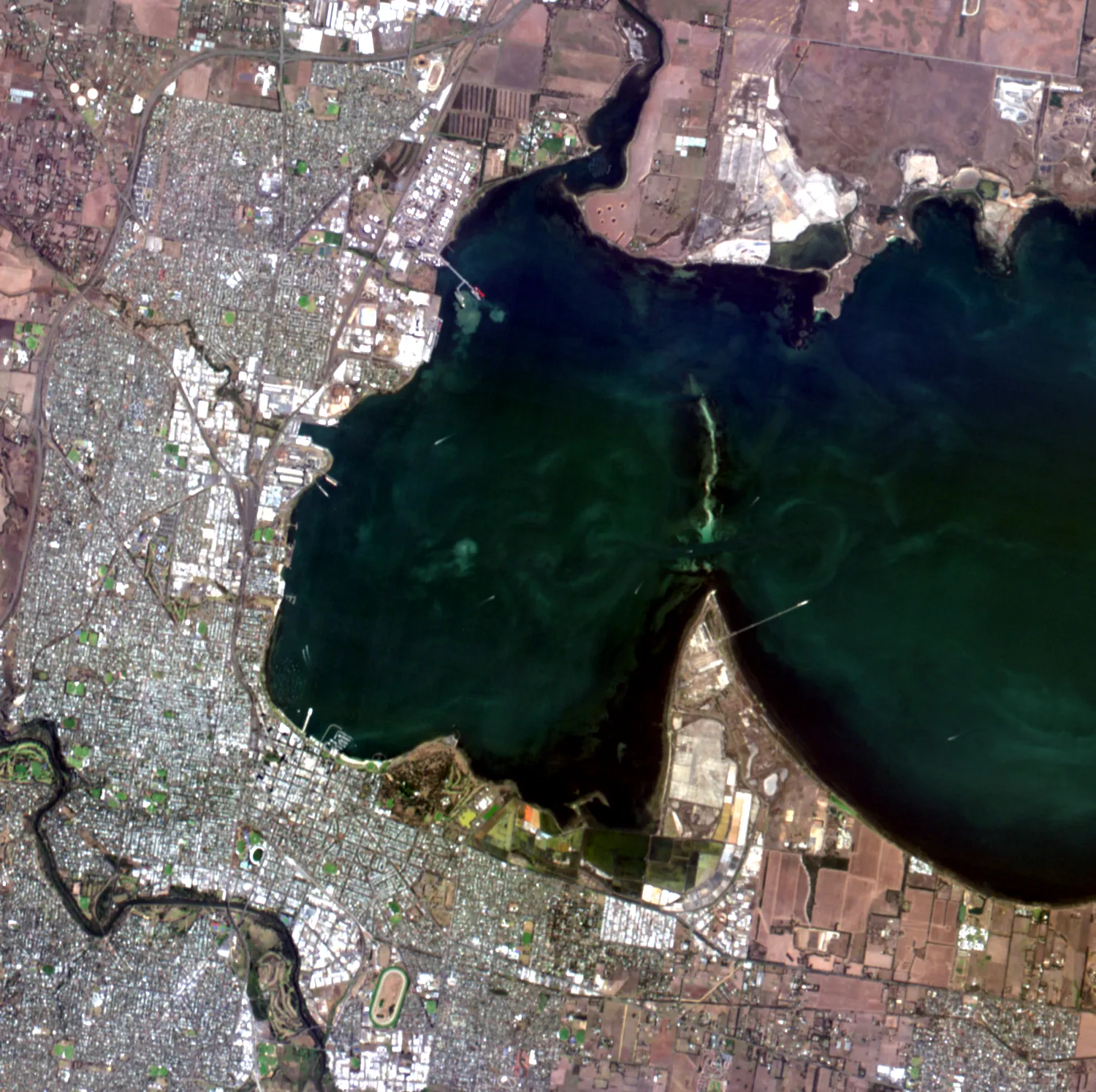
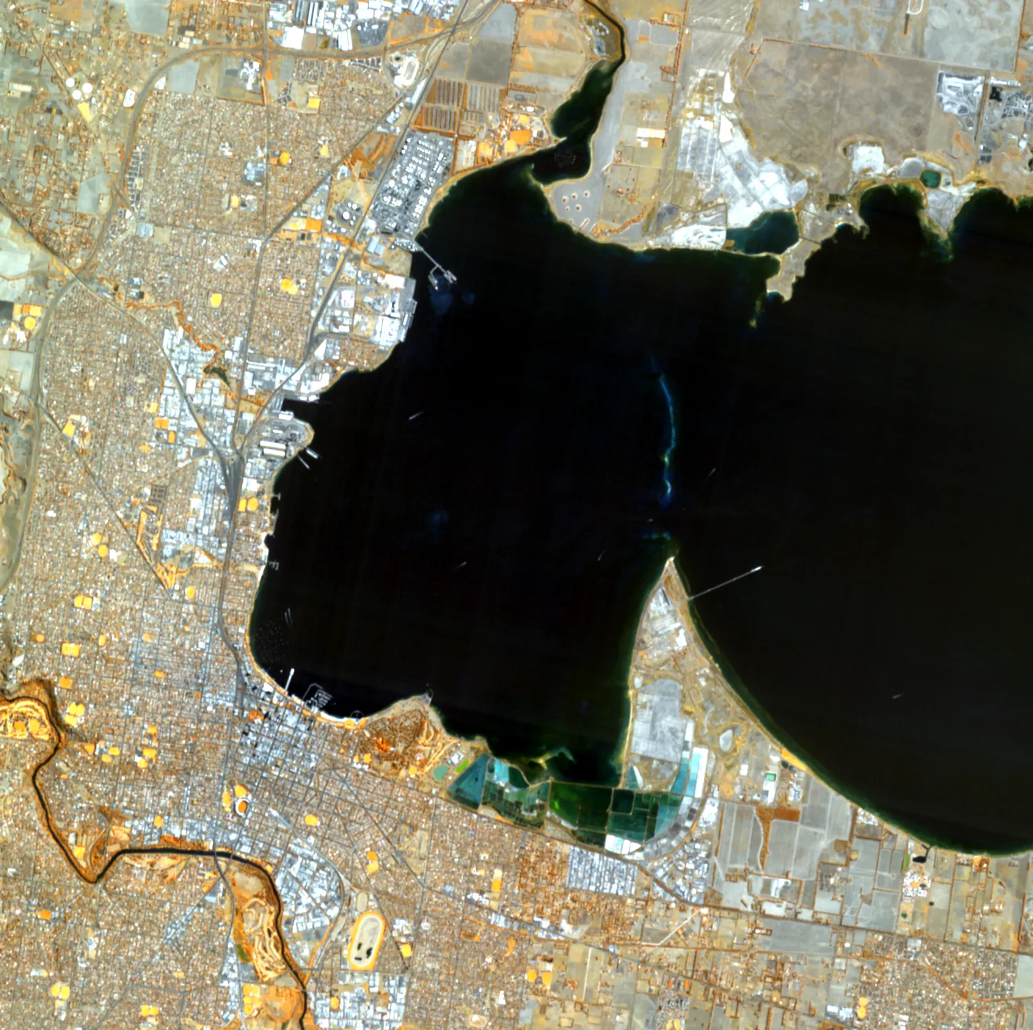
Drag the slider. In natural colour, Corio Bay is full of swirls: suspended sediment and plankton scattering green light. In the red-edge triplet the bay goes black, because water absorbs nearly everything past 700 nm, and the irrigated ovals and the old salt ponds at Moolap light up. Those are three of the 31 bands, and the other 28 are still in the file.
What a Hyperspectral Pixel Actually Contains
This is the figure the brochures never show, and it’s the reason to buy the product.
Four surfaces, 31 bands each
The turf curve is the textbook. Radiance sits at 22 units at 669 nm, where chlorophyll absorbs, then triples to 74 by 749 nm. That step is the red edge, and its exact position slides with chlorophyll content and stress, which is why ten bands across it are worth paying for and four are not quite. Dry pasture is nearly flat. Roofs are bright and slope gently down.
The water curve is the lesson about processing levels. Water should be dark at every wavelength, and past 700 nm it is. But at 445 nm Corio Bay reads 38, almost as bright as the turf’s 42. The bay isn’t that bright. The extra light is the atmosphere between the bay and the satellite, scattering blue into the sensor. Level 1B keeps it. Level 2A removes it.
The two levels differ in more than atmosphere. Wyvern’s L1B is 32-bit floating point radiance in W/(m²·sr·µm), in geographic WGS84, with pixels that are angular equivalents of 5 m, so the Geelong file’s pixels are 4.99 m wide and 5.01 m tall. L2A, released in February 2026, is surface reflectance as 16-bit integers with a 0.0001 scale factor, reprojected to UTM at a true 5 m, corrected with the 6S radiative transfer model and MODIS atmospheric data. If you’re comparing two dates, or matching pixels against a spectral library, L2A is the level you want. L1B is for people who run their own correction.
What Hyperspectral Satellite Imagery Costs
There is no public rate card for commercial hyperspectral that we know of, ours included. Our pricing page lists optical tiers. Hyperspectral is quoted per order, because four things move the number more than the per-km² rate does.
Minimum order area. Wyvern’s published minimums are 100 km² for standard tasking and 50 km² for premium tasking, with assured-capacity contracts sold by whole scenes. At 5 m pixels, 100 km² is 4,000,000 pixels by 31 bands: 496 MB as float32 L1B, 248 MB as uint16 L2A. If your site is 8 km², you are paying for 100.
Archive or tasking. Archive is cheaper and immediate, if a scene exists. Dragonette has been flying since April 2023, and as with any tasked constellation the archive is densest where customers have already tasked and thin elsewhere. Pera Portal shows what’s orderable over your polygon, with the price on the result, which is the fastest way to find out which case you’re in.
Processing level and processing chain. L1B is not a finished product, as the water curve above shows. At Geopera the chain runs on every order, orthorectification and atmospheric correction included in the rate, so the number on the result is the number on the invoice. Elsewhere, ask what level the quote covers. The general pattern for optical, where separately billed processing adds 30 to 80%, is laid out in our buying guide.
Licence. A single-user licence is the default quote. Organisation-wide use, public deliverables, and derived-product rights each need to be in writing before the order, not after. Regulators and clients almost always need derived-product rights.
Free data is not free of cost. It costs a place in the queue and a 30 m pixel, and then it costs an analyst’s week turning a 230-band cube into an answer. For a lot of projects that is still the right trade.
Free Hyperspectral Satellite Data: When It Is the Right Call
| Source | Pixel | Bands | Range (nm) | Access | The catch |
|---|---|---|---|---|---|
| EnMAP (DLR) | 30 m | 230 | 420 to 2450 | Free with registration via DLR’s portals | 30 km swath, tasking requests join a queue; 4-day off-nadir revisit |
| PRISMA (ASI) | 30 m | 239 | 400 to 2505 | Free with registration via ASI | Acquisitions are on demand, so archive over your site may be empty |
| EMIT (NASA, on the ISS) | 60 m | 285 | 381 to 2493 | Free via NASA Earthdata | ISS orbit: patchy coverage, nothing poleward of about 52° |
| Wyvern Open Data | 5.3 m | 23-31 | 445 to 869 | Free, CC BY 4.0, no registration, STAC | 109 fixed scenes as of September 2026, mostly L2A, and not your site |
The rule we apply, including against our own product: if the feature you’re chasing is in the shortwave infrared and 30 m pixels will do, download EnMAP or PRISMA first. Regional clay and iron-oxide mapping over a tenement is the classic case. Come to a commercial VNIR product when 30 m is too coarse, when you need a capture on a date of your choosing, or when the feature sits below 870 nm anyway, which covers most vegetation and water-quality questions.
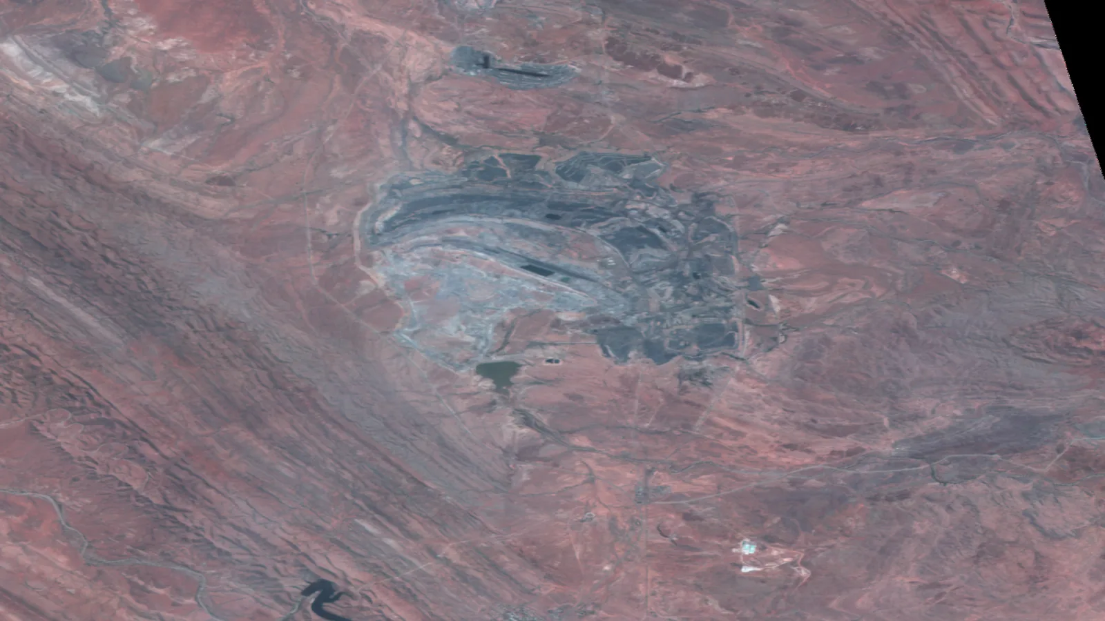
Wyvern’s open data programme deserves a specific mention, because it is the cheapest way to find out whether 5.3 m and 31 bands solve your problem before you spend anything. As of this month it holds 109 scenes, eight of them over Australia: the Kimberley, the Darling Downs, the Whyalla coast, the Leigh Creek coalfield in the northern Flinders Ranges (the image at the top of this page), and the Geelong strip used throughout this post. The catalogue is plain STAC JSON, so a script can list every scene in seconds.
Archive or Tasking, and What Turns Up
-
Find the wavelength of your target feature
Chlorophyll red edge near 700 to 750 nm, clays near 2,200 nm, iron oxides near 850 to 950 nm. It decides the sensor before anything else does.
-
Check the archive over your polygon
Pera Portal for Dragonette, with prices on results. DLR and ASI portals for EnMAP and PRISMA. This step is free and tells you whether tasking is needed.
-
Choose the level
L2A surface reflectance unless you run your own atmospheric correction. Ask for the processing chain in writing.
-
Task with thresholds
Capture window, cloud ceiling, and the minimum area you are being charged for, all on the order.
-
Receive and verify
A cloud-optimised GeoTIFF with 31 layers plus STAC JSON. Read the wavelength tags off the bands and check the footprint against your AOI.
One trap is worth recording for anyone handling their first delivery. The L1B GeoTIFF is north-up in degrees, so its pixel count bears no simple relationship to its area: the Geelong strip is 8,040 by 11,595 pixels, 93 million of them, of which 46 million hold data. Compute areas and file-size estimates from the data mask, not the raster dimensions. Each band carries its centre wavelength and full width at half maximum as GeoTIFF tags, and the band order is by wavelength, so read the tags rather than assuming a layout from the brochure. And the 12-bit radiometry is real: the sensor quantises to 4,096 levels, which is comfortably enough for the red-edge step and thin over dark water in the near-infrared, where the Corio Bay curve above sits between 8 and 12 units.
Delivery from us is a Cloud Optimized GeoTIFF, orthorectified, atmospherically corrected, with the same band stack Wyvern ships, so any of the 350-plus spectral indices we document can be computed from it directly. Archive orders are often delivered the same day. Tasking delivers when the capture window and the weather allow. Put a cloud ceiling on the order, because a capture without one can count as delivered at any cloud cover.
How We Handle Hyperspectral at Geopera
We have been a Wyvern partner since April 2025. Dragonette sits in Pera Portal next to WorldView-3, Beijing-3, SuperView and our own Perascope constellation, with archive search and tasking under one account, and the per-km² price on each result before you commit. Every order runs the same processing chain as our optical products, at no extra charge. Wyvern’s constellation grew by two satellites in 2025, Dragonette-004 and -005, with a sixth planned for 2026 on larger buses with more downlink, so archive density and tasking capacity are better than they were a year ago.
If you’re not sure whether the sensor fits, tell us the feature and its wavelength and we’ll say which sensor has it, including when the answer is free EnMAP data and not us. If you’d rather see a processed strip over your own site first, you can apply for a sample. We review applications, talk through the use case, and then process one.
Frequently Asked Questions
Can you buy hyperspectral satellite imagery?
Yes. In 2026 the commercial hyperspectral product available through Geopera is Wyvern’s Dragonette constellation: 5.3 m pixels, up to 31 bands between 445 and 869 nm, sold as archive scenes or new tasking through Pera Portal. Free hyperspectral data with shortwave infrared is available from EnMAP, PRISMA and EMIT at 30 to 60 m.
What is hyperspectral satellite imagery?
Hyperspectral satellite imagery records dozens to hundreds of narrow, contiguous spectral bands for every pixel, typically 5 to 30 nm wide, instead of the 4 to 16 broad bands of a multispectral sensor. The result is a full reflectance curve per pixel, which lets analysts identify materials, minerals and vegetation types by their absorption features rather than just their colour.
Is hyperspectral satellite imagery free?
Some of it. EnMAP (DLR), PRISMA (ASI) and NASA’s EMIT are free with registration, at 30 to 60 m pixels with 230 to 285 bands covering 400 to 2,500 nm. Wyvern releases 109 open Dragonette scenes under CC BY 4.0 at 5.3 m. Commercial 5.3 m imagery over a site and date of your choosing is paid.
What resolution is hyperspectral satellite imagery?
The finest commercial hyperspectral pixel in 2026 is 5.3 m, from Wyvern’s Dragonette satellites, covering 445 to 869 nm in up to 31 bands. Free government missions with shortwave infrared coverage operate at 30 m (EnMAP, PRISMA) and 60 m (EMIT). No hyperspectral satellite delivers sub-metre pixels, because each narrow band has to collect enough light to be worth reading.
How much does hyperspectral satellite imagery cost?
Commercial hyperspectral is quoted per order rather than listed, and the total is driven by minimum area, tasking tier and processing level. Wyvern’s published tasking minimums are 100 km² standard and 50 km² premium. Pera Portal shows the per-km² price on each Dragonette result before you order, and processing is included in Geopera’s rate.
It would be easy to read a one-line commercial menu as a reason to wait for the 2028 sensors. It’s the other way round. The buyers who will get value from 110 bands with shortwave infrared are the ones who spent the years before learning what 31 bands at 5 m do to their particular problem, on a scene they own, with a processing chain that already works. The learning is the expensive part. The pixels are not.