Backpropagating Through a Flood

Summary

• Our 2D flood-and-sediment model of the Bhote Koshi disaster runs on a GPU in PyTorch. That makes it differentiable: every output is a mathematical function of every parameter, with gradients available by backpropagation, straight through roughly eight thousand solver timesteps.
• So instead of hand-tuning the sediment physics, we made six parameters learnable and descended the gradient of the mismatch between simulated terrain change and the terrain change we measured from stereo satellite imagery.
• It reduced the misfit against the measurement by 59 percent in about half an hour on a consumer graphics card, and the calibrated physics came out sensible: finer sediment, lower critical shear, smoother flow than the hand-tuned values.
• Getting there took three failures worth documenting: infinite gradients at dry cells, exploding gradients through shock waves, and a 25-minute compilation from being greedy about kernel fusion.
• The strangest part predates the method. An earlier calibration target turned out to be wrong, and the model’s physics had visibly resisted it, putting sediment where the corrected measurement later said it belonged. Sometimes the model is arguing with your data for good reason.

This is the methods post in our Bhote Koshi series; the human context and the measurements live in the earlier posts. It gets more technical than usual, on purpose.

Why gradients, and why now

Calibrating a flood model has traditionally meant running it many times: pick parameter values, simulate, compare with observations, adjust, repeat. With four or six coupled parameters, the search space grows fast, every sample costs a full simulation, and the tuner’s intuition quietly becomes part of the model.

There is another way if your solver happens to be written in an automatic-differentiation framework. Ours is: we built it on PyTorch for GPU speed, back when the goal was just fast ensembles. But a solver written that way is secretly a very deep neural network, one whose “layers” are timesteps of the shallow-water equations with erosion, sediment transport, and deposition riding along. Ask for the derivative of the output misfit with respect to the erosion coefficient, and the framework will chain-rule its way backward through the entire flood.

This is a young but fast-moving corner of the field. Differentiable flood solvers built for exactly this purpose have begun appearing in the literature this year. Our contribution is small and practical: we did it to a real disaster, against a real satellite-derived measurement, and we are writing down everything that broke.

The setup

Six learnable parameters, in log space so they stay positive: an erosion coefficient, a critical shear stress below which the bed resists, a settling velocity, a speed threshold above which nothing deposits, the injected sediment concentration, and the Manning friction coefficient. The loss compares the model’s final bed-elevation change against the stereo-measured change on valley-floor cells, plus a weaker term matching flow heights at surveyed trimline points. One evaluation is a full simulation of the flood’s passage through the deposition reach, about eight thousand timesteps at 24-metre resolution.

One structural fix mattered before any gradient did. The original model domain ended at kilometre 42.5 of the corridor, which the stereo measurement revealed to be upstream of where the real deposit ends. The model could never have matched the measurement, because the measurement lay partly outside its world. The calibration domain now runs to kilometre 46.5. It is a good reminder that no optimiser can fix a domain boundary.

Three failures, in order

Failure one: infinite gradients at the water’s edge. The wave speed in a shallow-water solver involves the square root of water depth, and the derivative of a square root at exactly zero is infinite. Ninety-five percent of our domain is dry land sitting at exactly zero depth. The forward simulation was fine; the very first backward pass returned NaN for every parameter. The fix is an epsilon inside every square root, and the same medicine for the vector magnitude of velocity, whose gradient is undefined at exactly zero motion. If you take one line from this post into your own differentiable solver, take this one.

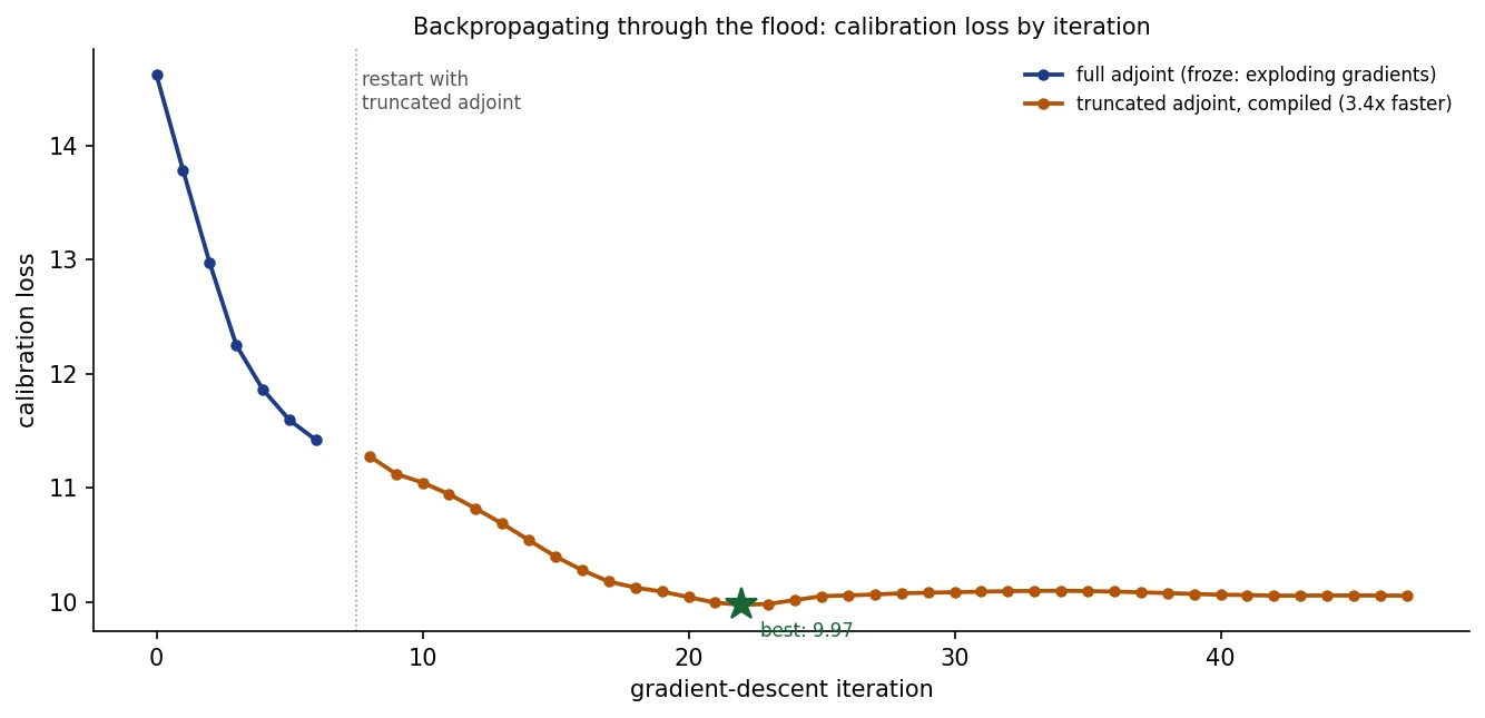
Failure two: exploding gradients through shock waves. With the poles patched, the descent ran for seven productive iterations and froze. Backpropagating through thousands of steps of nonlinear, shock-forming dynamics is the recurrent-network exploding-gradient problem in fancy dress: tiny perturbations to the flow amplify exponentially, and the gradients overflow. The cure is also borrowed from recurrent networks: truncation. We detach the fast, chaotic flow state every sixty steps, while keeping the slowly accumulating bed-elevation chain, the thing the loss actually measures, differentiable end to end. Gradients through the morphology survive; gradients through the turbulence-adjacent chaos are cut before they can explode. After this change, not a single gradient overflowed in forty iterations.

Failure three: greed at compile time. To speed things up we asked the compiler to fuse all sixty timesteps of a segment into one giant kernel graph. Twenty-five minutes later it was still compiling and the GPU had done nothing. Compiling a single timestep instead takes seconds and captures nearly all the win, because the benefit is fusing the forty small operations inside a step, not gluing steps together. With that, plus moving the inflow lookup out of the inner loop, an iteration dropped from 174 seconds to 37.

What the flood learned

The descent cut the terrain-change misfit by 59 percent, most of it in the first fifteen iterations. The calibrated parameters tell a coherent physical story. Critical shear fell from 250 to 150 pascals and the settling velocity from 0.15 to 0.054 metres per second: the sediment behaves finer than we had assumed, staying in suspension longer and travelling further down-valley before dropping, which is exactly the correction the measured deposit demanded. Manning friction fell from 0.050 to 0.034, echoing a result we found earlier by a completely different route, that this flood moved like water, not like a viscous debris slurry. And total modelled deposition in the reach fell from 21 million cubic metres to about 5, from four times the measured scale to roughly matching it.

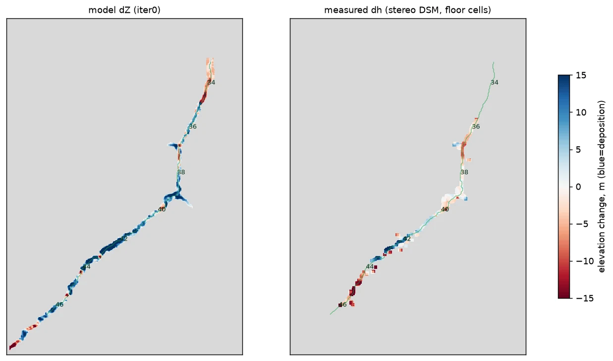
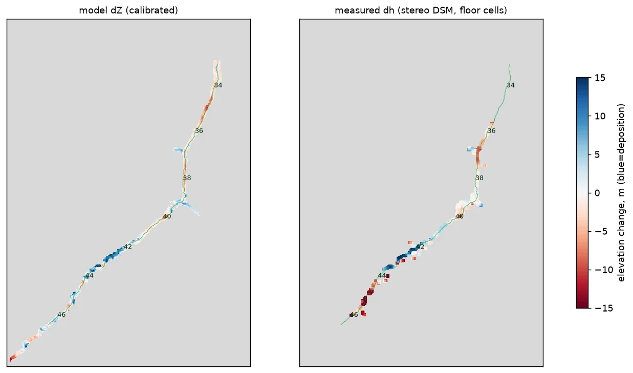
Where it stopped is as informative as where it got. After iteration fifteen the loss went flat while parameters drifted: friction pinned against its lower bound, critical shear wandering without improvement. That is what exhausting a parameterisation looks like. Six numbers cannot express that friction differs between bedrock gorge and gravel fan, or that erodibility varies along fifteen kilometres of valley. The obvious next step, spatially varying parameter fields with appropriate regularisation, is exactly what gradient-based calibration is uniquely equipped to handle, and exactly what grid search never could.

The model that argued with its data

One thread from earlier in this series belongs in the record here. Before the stereo measurement existed, this model was calibrated against a sediment map that later proved wrong, made with a parallax method whose viewing-geometry assumption did not hold. That target put the main deposit five kilometres upstream of where it really is. The remarkable thing, visible only in hindsight: the model never fully complied. Its physics kept carrying sediment through the gorge and dropping it at the valley opening, centred within one bin of where the corrected measurement eventually placed the real deposit. The calibration pulled; the shallow-water equations pushed back.

We do not want to romanticise this. A model can be wrong in ways that also resist your data. But it is a concrete argument for keeping real physics inside learned systems: the structure of the equations encoded knowledge about where sediment can and cannot come to rest, knowledge that survived contact with a corrupted calibration target.

An honest appendix: the measurement that refused

Not everything we tried this week worked, and one null result deserves recording. Landsat 9 imaged the flood mid-event, and the instrument’s spectral bands are captured a fraction of a second apart, a lag that has been used to measure ocean currents and drifting river ice. We attempted to measure the flood’s surface velocity from that inter-band displacement. The machinery worked beautifully, down to a detection floor near half a metre per second, and measured the moving floodwater at essentially zero. The reason is structural: on a river a few pixels wide, image correlation locks onto the static banks, not the moving water between them. The technique wants open water or discrete floating objects, and a Himalayan river in a gorge offers neither. We publish the negative so the next person can spend their afternoon on something else.

Code for the simulation lives in the open reconstruction repository, alongside the terrain data this calibration learned from.